
Loss aversion means a loss hurts about twice as much as an equal gain pleases. Offered a fair coin toss to win 200 dollars or lose 100 dollars, many people accept it. Offered 100 dollars to win against 100 dollars to lose, most refuse. Daniel Kahneman and Amos Tversky described this pattern in 1979 as part of prospect theory.
- Loss aversion is a weighting rule, not a feeling about risk in general.
- The reference point decides what counts as a loss or a gain.
- The value curve is flat for gains and steep for losses.
- In mixed bets the median need is about double: 100 loss needs about 200 gain.
- It drives the endowment effect, sunk-cost thinking and status-quo preference, but it is not the same as any of them.
- Its strength shifts with context and background, so no single number fits all.
What loss aversion means
Loss aversion is the tendency to weigh a loss more than an equal gain. The classic phrase is losses loom larger than gains, from Kahneman and Tversky in 1979. It is a cognitive bias, not a perception error and not an illness.
The reference point is the key. A change counts as a loss or a gain only against a starting point. That point can be what you own now, such as your balance today. It can also be what you expect, such as a sales target or a grade you aim for. Prospect theory differs from older utility theory here: it judges the change from the reference point, not the final wealth. The English overview of loss aversion states the same point with the same 1979 source.
Loss aversion is not risk aversion. Risk aversion means you value an uncertain outcome below its expected value. Loss aversion means you weigh the loss part of an outcome more than the gain part. Keep the two apart in an exam answer.
If you know cognitive biases as a family, place loss aversion with the biases that shape judgment, such as anchoring bias. It is a bias in how you value, not in what you see.
The curve behind it: gains flat, losses steep
Kahneman and Tversky proposed a value function that treats gains and losses in a different way. The function has three traits. It is defined as a move away from the reference point. It is concave for gains and convex for losses. It is steeper for losses than for gains, and steepest near the reference point.
Concave for gains means each extra dollar adds less value than the last. Convex for losses means each extra dollar of loss adds less pain than the last, but from a higher base. Diminishing sensitivity follows: the gap between 100 and 200 feels larger than the gap between 1000 and 1100, on both sides.
Risk behavior flips at the reference point. Faced with gains, people turn cautious: they take 100 dollars for sure over 200 dollars with 50 percent chance. Faced with losses, people turn bold: they take an uncertain large loss over a sure small loss, because they hope to escape the loss. This flip is a standard exam question on prospect theory.
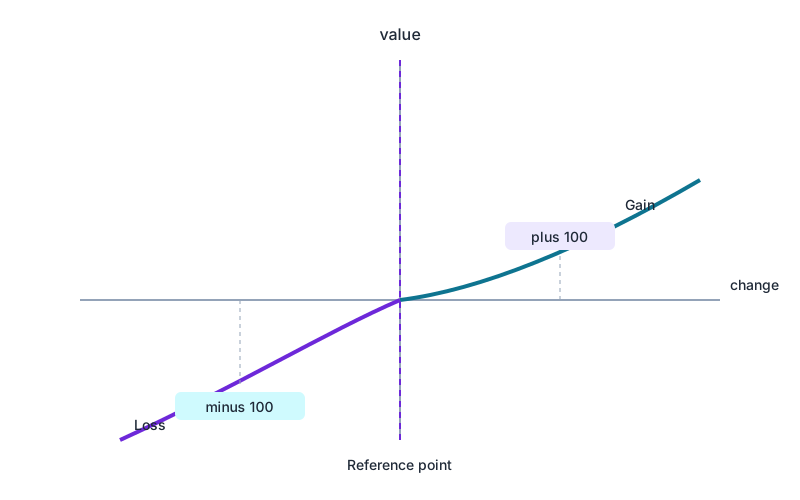
The numbers come from later estimates. Tversky and Kahneman reported in 1992 a median loss-aversion factor of 2.25. The curvature was 0.88 for gains and for losses. The tasks were small unpaid lotteries with students. See Advances in prospect theory. A 2024 meta-analysis in the Journal of Economic Literature finds mean values near 2. It judges 2.25 as a little high. See Meta-analysis of Empirical Estimates of Loss Aversion. Use about 2 as a rule of thumb, with a range of 1.5 to 2.5, and name it as a median, not a law.
The 100-dollar test and two studies you should know
The simplest test is a mixed lottery. Ask: what smallest gain G makes a 50-50 chance of G against a 100-dollar loss worth taking. The common answer is near 200 dollars. The ratio sits near 2 in many samples, with a spread of 1.5 to 2.5. The loss needs about double as cover.
The second study is the mug study by Kahneman, Knetsch and Thaler from 1990. Sellers with a mug asked about double the price that buyers without a mug would pay. From the seller view the mug counts as a loss against the reference point of owning it. From the buyer view it counts as a gain. The same object gets two prices, set by the reference point. The loss aversion overview reports the mug and chocolate trials. It rules out transaction costs, confusion and bargaining habits as other causes. It also rules out income effects and trophy effects.
The third case is taxi drivers with weak daily pay, studied by Colin Camerer in the 1990s. Drivers set a daily income target. On days with high demand they stopped early, on days with low demand they drove long. By pure income logic the reverse would pay: drive long when demand is high. The daily target as reference point explains the pattern. Treat it as an illustration of a target as reference point, not as proof that all drivers act this way.
For an exam, link each case to one idea. Lottery tests strength. Mugs test owning as reference point. Taxi tests a goal as reference point.
Four cases, one pattern: how to keep them apart
Loss aversion explains many patterns, but it does not replace them. Textbooks name the endowment effect, the sunk cost fallacy and status-quo preference as outcomes on the behavior level. Keep them apart with one question: what is the person weighing now.
| Case | The question behind it | Example |
|---|---|---|
| Loss aversion | Does the loss weigh more than the same gain | 100-dollar loss needs 200-dollar gain as cover |
| Endowment effect | Does owning set the reference point | Seller asks double what buyer offers |
| Sunk-cost thinking | Do past costs count, though they never return | Hold a losing share because much was paid |
| Status-quo preference | Does the person stay, because change counts as loss | Refuse extra pay for fewer holidays |
The stock case shows the chain. Investors sell winners early and hold losers long, because selling writes the loss down. They then search only for news that supports holding. That is confirmation bias. And they stay with the first choice to avoid conceding that it was wrong. That pull comes from cognitive dissonance. Loss aversion is the engine, the other two keep the car on the road. Name each part in an answer.
When the effect gets weaker
Loss aversion is strong, but it is not fixed. Walasek and Stewart ran five experiments in 2015. They showed that the same bet is judged in a different way when the bets seen before shift. Context moves the scale, as a room feels warm or cold based on where you stood before. The effect does not vanish, it depends on comparison. The paper ran in the Journal of Experimental Psychology: General, volume 144, pages 7 to 11.
People differ as well. Gachter, Johnson and Herrmann found in 2010, with an update in 2022, no clear gap between men and women. Loss aversion rose on average with age, holdings and income, and fell with schooling. The paper ran in Theory and Decision, volume 92, pages 599 to 624. For your answer, never give 2.25 as a fixed value for all. Give median, range, and the role of context and schooling.
A note on debate helps you read sources with care. Some researchers argue that inertia explains these patterns better than gain-loss weighting. They point to status-quo persistence, the endowment gap and safe-over-risky choices. Gal argued this in 2006 and with Rucker in 2018. Others show that loss aversion has moderators, but that reports of its death go too far, as Mrkva, Johnson, Gachter and Herrmann did in 2020. The behavioral economics guide lists both sides. Expect the factor to move, not to vanish.
How to remember it for the exam
Make a list in Psychology World named Decision. Save these five terms: loss aversion, prospect theory, endowment effect, sunk cost fallacy, status quo. Learn them as a group, not alone.
Proceed in this order. Read the definition aloud. Cover the examples and name one case for each: lottery, mug, taxi, share, holiday. Quiz yourself with flashcards. Then use the typing game, because typing exposes mix-ups between endowment and sunk cost fastest. Repeat the list after two days. This turns lookup into recall, with no new system to build.
Frequently asked questions
What is loss aversion in simple terms
Loss aversion means a loss of 100 dollars hurts more than a gain of 100 dollars pleases. That is why many people need about double the gain to accept a 50-50 bet with a loss in it.
How large is the factor in loss aversion
The median sits near 2. The early estimate by Tversky and Kahneman from 1992 names 2.25 with a curvature of 0.88. Later work finds a range of 1.5 to 2.5 and meta-analyses lean to values near 2.
What has loss aversion to do with prospect theory
It is one part of prospect theory by Kahneman and Tversky from 1979. The theory values gains and losses from a reference point. The curve is concave for gains and convex for losses. Its path is steeper in the loss zone.
What is the difference between loss aversion and the sunk cost fallacy
Loss aversion weighs a future gain against a future loss of the same size. The sunk cost fallacy counts past costs that never return. Loss aversion can feed sunk-cost thinking, but it is not the same thing.
Is loss aversion equally strong for all
No. Its strength depends on context, such as which bets you saw before. It rises on average with age, holdings and income, and falls with schooling. Gachter and colleagues found no clear gap between men and women.
Sources
- 1.Kahneman, D. and Tversky, A. (1979). Prospect Theory: An Analysis of Decision under Risk.
- 2.Tversky, A. and Kahneman, D. (1992). Advances in prospect theory: Cumulative representation of uncertainty.
- 3.Brown, A. and others (2024). Meta-analysis of Empirical Estimates of Loss Aversion.
- 4.Loss aversion in the English Wikipedia, read 4 November 2026.
- 5.Pilat, D. and Krastev, S. (2019). Loss aversion at The Decision Lab.
- 6.Loss aversion at BehavioralEconomics.com, updated 4 December 2024.